Introduction

With billions of computations per second, our brains are the most complex and intelligent entities the world has ever known. So intelligent, in fact, that we’ve been able to design other entities to do work for us — computers. With the rise of automated, electronic technology, it’s particularly thought-provoking to compare brains with the processors that now control our future. We’ll see that their differences complement each other, perhaps by design, and take a look at what happens when we blend them together.

Let’s begin by thinking about what we as humans already know about brains and computers. One major difference between us and computers is consistency in output — a computer always displays a “2” the exact same way on its screen, but if humans write a full line of the number “2”, our numbers might not always look the same. In addition to consistent output, a computer more reliably maintains the integrity of data long-term, while our brains modify memories slightly whenever we access them [1]. However, the brain has its strengths in robustly interpreting varied input: when reading handwriting, we can often recognize badly formed letters and very quickly learn to pick up on patterns in the writing. Computers take much longer and perform far worse at this; they cannot learn patterns in the same way that we can. Another example of this is ELIZA, one of the first ever chatbots, designed to speak to people as a psychotherapist. If you try speaking with it, you’ll notice that it has trouble carrying conversations and adapting to the wide variety of responses we can give it. A clear trend that emerges is that computers are excellent at reliably performing specific, repetitive tasks that are tedious for us to complete (for example, storing and copying large amounts of data from one location to another). On the other hand, the decision for which task it should perform, and exactly how, is left to human brains, which think less specifically and are adept at recognizing, adapting to, and generalizing broader “big-picture” patterns.

Building Blocks

Computers are made of transistors, electronic switches controlled by a single input and an output that is “all-or-nothing” [2]. This on or off behavior of transistors forms the bedrock of binary computing, and these two different states, represented by the logic values of 0 and 1, constitute all data and all possible computations. When combined in certain configurations, transistors create logic gates, which are computers’ fundamental unit of computation. Logic gates can therefore be seen as a kind of analogue to neurons. Examples of logic gates include those that do basic computations on a very small number of binary inputs to produce outputs, such as the “and” logic gate, made of two transistors in series, and the “or” logic gate, made of two transistors in parallel. In the case of an “and” gate, if either transistor is off, electricity cannot flow through the gate, thus both are required to be on for a signal on one side of the gate to pass through to the other side. In contrast, the “or” gate is set up such that an on signal at the start can pass through either of two transistors to pass through the gate, such that if even one is on, the “or” gate outputs on.

Aside from operations with logic gates, computers can also configure data storage in binary via the positioning of magnets. This provides a more robust method to store data that doesn’t rely on a constant flow of electricity, and adds to a computer’s reliability. One unit of memory representing a 0 or 1 is a bit, and 8 bits next to each other make a byte that can represent 28 or 256 different states. One application of byte storage is the representation of digital color. Computers use one byte to represent the light intensities of each of the three primary colors, red, blue, and green as a number from 0 to 255. These three bytes then can be used to represent all of the colors in the color wheel. Bytes are the fundamental way all computers store data, and nearly all computation we use today ultimately comes down to these 0s and 1s.

The fundamental building block of the brain is the neuron. These cells are highly interconnected, receiving inputs from and providing outputs to potentially thousands of other neurons. Neurons receive inputs via synaptic potentials, summing up varying strengths of both excitatory and inhibitory signals from huge numbers of presynaptic neurons. This gives their computations a graded component that pays attention to the magnitude of a stimulus rather than solely its presence or absence. Neurons only fire an action potential if the sum of their inputs crosses a threshold, and this action potential is an all-or-nothing response, giving their signaling a binary component as well. These binary signals become graded inputs for a postsynaptic neuron via synapses at its axon terminals. Stronger and more numerous synapses with a postsynaptic neuron result in a larger input to it from the presynaptic neuron for the same action potential. Over time periods longer than individual spikes, neurons often have a baseline firing rate, and change their firing rates in a graded manner. Different neurons express these graded and binary components to varying degrees, allowing for great versatility in the types of signals represented. Furthermore, many neurons have the versatility to adapt the range their signals represent, and do so over very short periods of time [3]. These different characteristics of the building blocks of the brain and the computer help explain their differences in overall processing.

Things Get Messy

Despite the major differences between neurons and computing units, all signaling systems have an intrinsic component of variability in their signaling, called noise, and this in large part explains the differences in reliability and adaptability between brains and computers. Because chemical processes are random, noise is omnipresent throughout neural signaling [4]. This noise reduces reliability of neural signals, but it is also precisely why neurons are more adaptable than transistors. A familiar example of biological molecules reducing reliability while improving adaptability is via genetic mutations. While some are caused by radiation or toxic chemicals, others take place due to seemingly random changes in organic molecules. Given that the action potentials of neurons are generated by these same types of molecules, it is unsurprising that they also contain a component of noise that can sometimes corrupt signals. However, just as the mutability of DNA allows mutations beneficial for fitness that lead to evolutionary adaptation, a slightly noisy signal in the nervous system could be what allows for the discovery of the optimal processing pattern and response to a stimulus. Electronic systems are certainly not immune to the issue of noise, but the strategy of segregating signals into zeros and ones, known as digitization, allows computers to be very reliable. This reliability of the most basic level of signaling in computers may be a reason why computers perform tasks with greater precision.

The properties of the units making up brains and computers account for their larger characteristics. We’ve established that due to increased randomness in its neurons, the brain has lower reliability at certain tasks while also having greater adaptability; computers produce more definite, consistent output. In addition, the fact that neurons adapt over very short periods means that our sensory experiences are measured in relative rather than absolute units, and we can’t always compare them to each other. An example of this is clearly visible when your eyes adjust after leaving a dark room — the baseline firing rate of the relevant neurons now corresponds to a different light level than before. Computer cameras are less adaptable, so they can detect and report absolute levels of light, but if you’ve taken pictures at night, you’ll know they have a hard time extracting features of the space around them. Thus, while our experiences are less comparable to each other and our neurons don’t reliably produce the same firing rate for a certain light level, they do allow for better adaptation and performance under certain conditions.

Despite these differences, neurons and transistors still have very important similarities. They both turn electrical signals on and off quickly, allowing for an extremely fast speed of processing at billions of computations per second. Both are also extremely small, with most central nervous system neurons between 200 nm to 20 μm, and transistors currently at about 5-25 nm, or about 10-60 atoms wide [5][6]. In addition, both neurons and transistors receive inputs and produce outputs, allowing us to model them mathematically with functions and statistically analyze them.

The Brain’s Wild Card

Aside from the differences between the individual units making up the brain and the computer, these two systems also differ greatly in their architecture. Different regions of a computer are specialized, with different parts of it storing memory, performing computations, managing the display, and accepting input from the user. Further, because transistors display reliable signaling properties, information can be transmitted with good fidelity through just a few connections. On the other hand, the brain displays many characteristics of processing that is distributed across larger populations of neurons, and this is the subject of an up and coming field in neuroscience called population dynamics.

A major rationale for studying dynamics across neuron populations is that neurons in the brain do not always fire in response to a single stimulus. For example, single neurons in the entorhinal cortex, a region thought to be involved in spatial navigation, fire in response to a variety of events during a variety of tasks [7][8][9]. Neurons in the prefrontal cortex, which is thought to play a role in planning and problem solving, can respond to visual stimuli during visual tasks in non-human primates [10]. Such cases suggest that single neuron recordings may not always be the most illuminating in characterizing the functions and firing patterns of brain regions. However, despite the fact that neurons in certain brain regions may not reliably fire in response to one stimulus, populations of neurons can reliably fire and transmit information via synchrony. Because each individual neuron manipulates a small aspect of population firing, this signal can be graded, and is relatively stable to random fluctuations in neuron signaling, enabling the nervous system to produce reliable signals and outputs. Thus, in a single region, individual neurons can respond to many signals, and many neurons can together represent one signal.

Similar neural signals can also be processed in multiple regions. In a task where mice made a choice to turn a wheel either left or right in response to a visual stimulus, researchers recorded from a wide variety of neurons throughout the brain [11]. They found neurons predicting a response to the stimulus (i.e. the mouse was engaged rather than disengaged with the task) in nearly every region recorded, and neurons predicting which direction the mouse would turn the wheel were found in both the forebrain and midbrain regions. These findings suggest that the signals encoding responses and choice are far from being localized to one region of the brain, and that it’s entirely possible that computations could be done in a distributed manner as well [11]. New methods in neuroscience and computer science are allowing us to concurrently record from many more neurons across many brain regions to better understand the neural code.

Technology Upgrades

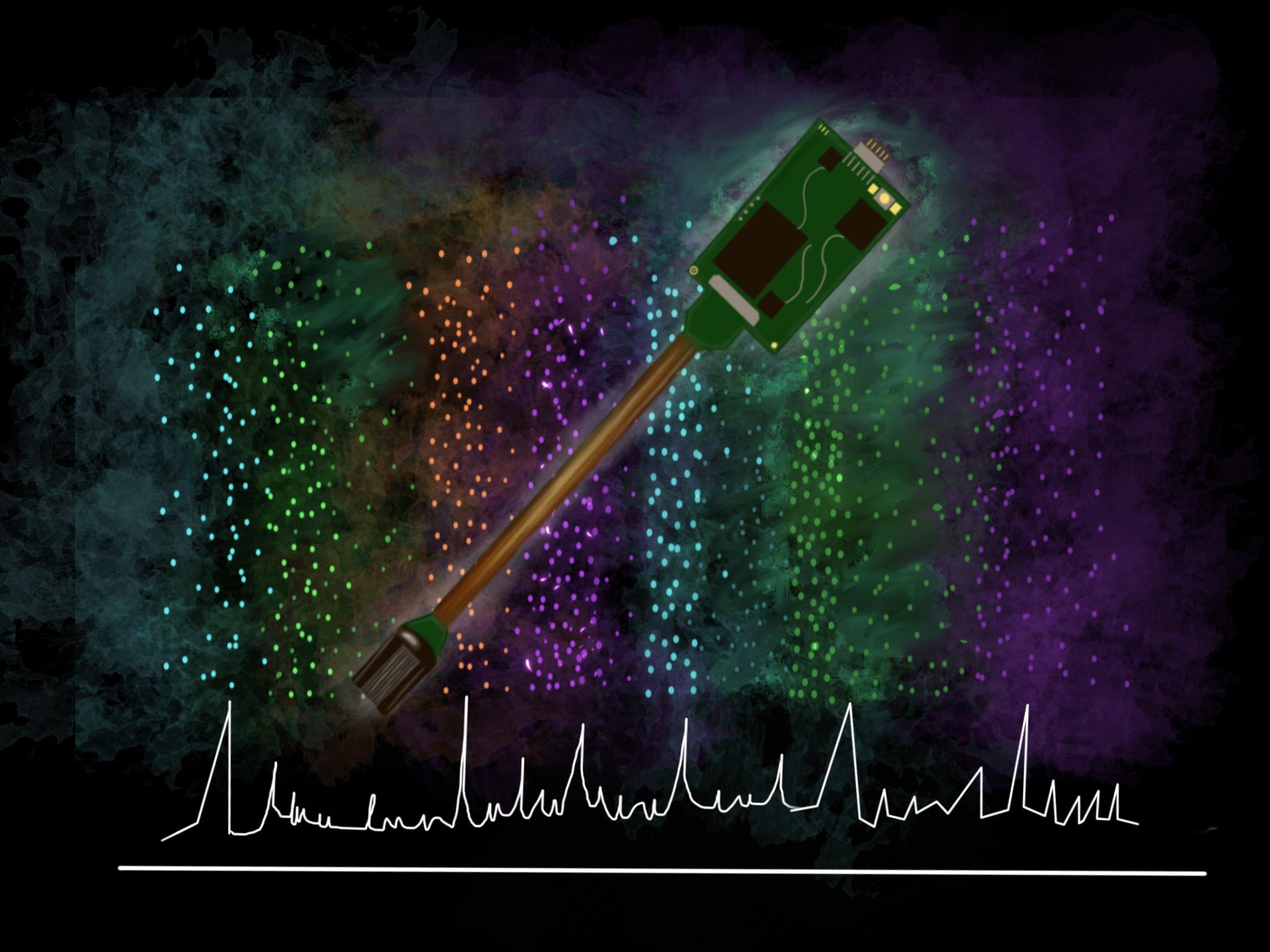
To understand population dynamics, neuroscientists have developed new tools and techniques to better visualize the activity of large numbers of neurons. One commonly used technique is electrocorticography (ECoG), which involves placing an array of electrodes on the cortex of the brain, but it isn’t able to detect action potentials of individual neurons [12]. In the last decade, micro-ECoG electrode arrays have been developed to gain much better spatial resolution [12]. Another very new device that is currently revolutionizing neuroscience is the Neuropixel probe. This next-generation electrode array has such dense recording sites that it can fit 384 channels onto a shank that is 1 centimeter long and less than a tenth of a millimeter wide [13]. It is already being used in neuroscience labs around the world to visualize the activity of hundreds of neurons at once. Both of these devices will be particularly useful in studying population dynamics, as they provide scientists with huge troves of data on simultaneous neural firing patterns during various animal behaviors.

Conducting large-scale analyses on this type of data forms a major frontier in the future of neuroscience. One approach that researchers take is to map the population’s firing over time into “neural state space” [10][14]. Looking at a simple population of two neurons, we can create a graph with the firing rate of one neuron on the x-axis and the firing rate of the other on the y-axis. The population’s “state” would be determined by the firing rates of each of the two neurons, and it would correspond to a point on that graph whose coordinates are those two firing rates. Over time, as the firing rates of these neurons change, the point representing the neural population’s state moves around this two-dimensional “space,” and adding more neurons adds more dimensions to the space. Scientists can scale this approach up to, say, the hundreds of neurons recorded from a neuropixel to map a population’s state in a very high dimensional space, and observe how the population moves in neural state space during various activities and behaviors. Mathematical techniques allow us to reduce the dimensionality of the neural state space to a low dimensional space that illuminates which sets of neurons in the population change their firing rates the most in response to various stimuli, allowing us to identify certain sets of neurons by their responses. This approach holds great promise for helping us understand neural populations in which a variety of neurons respond to a variety of different stimuli [14].

In addition to population dynamics, researchers have also developed methods of visualizing distributed processing. One method, called wide field calcium imaging, involves fluorescent dyes that light up in response to increased calcium concentrations from neuron firing [15]. These dyes can be injected or genetically engineered into certain populations of neurons, and we can visualize their activity by recording a video of this fluorescence over time. This technique cannot always provide us with absolute levels of activity, as it mainly deals in relative terms, and sometimes can be difficult to interpret [15]. Researchers at the University of Washington are working on developments to improve our efficacy at inferring firing patterns from this data [16]. In the meantime, it still provides us with a useful way to view the activity of neurons across the brain all at once.

These methods will be critical to further understanding the way the brain performs complex computations, both at a population level and at a systemic level. While these are already revolutionary, there is no doubt that they will continue to improve even as new ones are developed. We have witnessed exponential progress in the last decade, and the next few hold even more potential.

Neural Mimicry in Artificial Intelligence

In addition to observing the brain, we can also understand it by simulating it. Artificial neural networks, computer models of the brain, were first piloted decades ago as a type of machine learning, but scientists lacked the hardware to perform the expensive computations they require. In today’s day and age, however, neural networks can be trained in a matter of hours on a typical laptop, and even faster on industrial level supercomputers. The emergence of artificial neural networks brings with it an interesting question: how similar are these to our “real” neural networks, and how do the differences in their architectures lead to differences in output and behavior?

Like the brain, neural networks are made of neurons, single units that integrate many inputs and produce a single output. It may not be so surprising, then, that mimicking the functions and properties of biological neurons can be a successful strategy for producing effective neural networks. In 2012, one group of computer scientists attempted to replicate single-neuron adaptation with a special type of function in AlexNet, a neural network that classified the contents of 1.2 million images into 1,000 different categories [17]. They found that this significantly reduced the number of misclassifications to about 15%, nearly 10% better than the next best network. Neuroscientists have observed that biological neural networks do large amounts of pruning, or dropping of less important synapses. AlexNet used a new technique called dropout, which mimicked this technique and dropped connections that did not significantly sway the network’s choice of classification [17]. In 2015, Google’s GoogLeNet also implemented a strategy of dropping out up to 70% of neurons in some portions of its network, which contributed to a record low error of 6.67% on the same dataset [18]. Neural networks’ applications are impactful and wide-ranging: a Google offshoot recently developed a network called AlphaFold that predicts the structure of a protein from its amino acid sequence. Their model has nearly doubled our accuracy in these predictions, showing the powerful and wide-ranging applications of neural networks when applied to computational problems — in this case, one of the oldest in biology [19].

However, there are still many aspects of real neurons that artificial neurons do not yet reflect. The neurotransmitters of biological nervous systems have a much richer variety of signaling between neurons that isn’t reflected in artificial neurons. Artificial neurons usually contain noticeably fewer inputs than the sometimes hundreds of thousands present in biological neurons. Finally, while AlexNet mimicked the pruning of biological nervous systems to its advantage with dropout, computer scientists are still attempting to optimize what kinds of connections a network should drop, how many, and when. Neural networks are a very hot topic in computer science today, and some of these questions will likely be answered during our lifetimes.

The fact that neural networks conserve some properties of biological ones raises the question of how similar these systems are internally. To explore how these artificial neural networks compare to biological neural networks, a group of scientists at the University of Washington conducted a study on AlexNet to look for parallels between its artificial neurons and those of the monkey visual system, which has neurons that detect contrast to view points, lines, and at later levels, shapes [20]. In AlexNet, the researchers found artificial neurons that increased their firing in response to seeing objects whose edges had specific types of curvatures, regardless of the location of the shape in the visual field. These firing properties are hallmarks of neurons from a region in the monkey visual system, called V4, suggesting that this subset of neurons could play a functional role in AlexNet similar to that of V4 neurons in the monkey’s visual system [20]. Further research will help us better understand the similarities and differences between the computations in brains and neural networks.

It’s astounding that despite all of the differences between artificial and biological neural networks, we see such similar elements in both of them. While this is an ongoing area of research, it’s very possible that as artificial neural networks improve, we’ll find that they optimally solve the computational problem of vision in the same way that our own brains do. If so, this might imply that our brains detect objects in the world with optimal efficiency. On the other hand, neural networks may even outperform our brains at some point, being able to detect objects with greater precision (cameras can already see farther than we can, after all), more reliably, faster, and with less spatial overhead. If we develop the right systems, technology, and understanding of the brain, we may be able to remodel our own brains on these efficient systems and repair or enhance our own visual capabilities.

When Systems Collide: Brain-Computer Interfaces

Artificial neural networks are a huge step forward in the field of machine learning, but we may also want to translate them into physical systems beyond software to allow them to meaningfully interface with our own brains. That synergy could be one of the most powerful computational systems the world ever sees, and at the moment, it is helping people with lost limbs use prosthetic ones.

Given how long the idea of neural networks has been around, it’s not surprising that the idea of using them in brain-computer interfaces has been around for a long time as well. But now that we have the computational resources to implement them, we see that training an artificial neural network to interpret signals from a real one has been surprisingly effective [21]. In addition, researchers at the University of Washington found that networks trained on individual spike data improved their performance faster than those trained on neural data averaged over time, which may be indicative of the importance of individual neurons’ temporal coding [22]. This type of research helps improve patient outcomes, but also helps us understand what the neural code really is and what aspects of it store information.

In addition to creating neural networks that record from the brain and interpret its signals, it may also be useful to create systems that directly connect back to it in a way it can understand. We have already seen that the brain is extremely adaptive and can learn to see from echolocation [][24]. In 2020, a group of scientists engineered a hybrid synapse that interfaces with the brain and receives neurotransmitters from biological presynaptic neurons [25]. In particular, their hybrid synapse includes mechanisms that remove dopamine from the synaptic environment shortly after it is released, similar to the process of neurotransmitter reuptake. While this system has only been piloted in cell cultures so far, they were able to simulate long-term potentiation in this hybrid synapse, which represents a major breakthrough in the development of such an interface [25]. Further advances in this domain could lead to neuron-like elements used in hardware alongside or in replacement of transistors.

Conclusion

The brain and the computer are systems that can conduct very similar operations, but their inner architecture and functions are very different. In many ways, the differences between the brain and the computer complement each other: one is robust, the other more adaptable. This is perhaps why computers are so useful to us — they are able to do a wide variety of operations that we find difficult or time-consuming. Together, the brain and the computer are changing the world faster than they ever could separately. As we learn more about the brain with new techniques in neuroscience and develop new systems that integrate the brain and computer even more tightly, we will likely see technological and academic advances made even faster.

As we consider these technological advances, future work in this field raises a number of philosophical questions: What makes something a brain, and what makes it a computer? What do we call a system that incorporates the elements of both? We are also reminded of ethical standards: as our technology improves, the advances made must be communicated to the public effectively, and appropriate measures must be taken to ensure that science does not leave ethics by the wayside. Further, we must acknowledge the possibility that the systems we create may become sentient themselves — what rights and abilities should they have? As always, neuroscience and computer science raise a number of unanswered questions. The fields’ unbelievable progress will continue to amaze us in the years to come.

References

[1] Agren, T. (2014). Human reconsolidation: A reactivation and update. Brain Research Bulletin, 105, 70-82. doi:10.1016/j.brainresbull.2013.12.010

[2] Tsividis, Y., & McAndrew, C. (2011). Operation and modeling of the MOS transistor (3rd ed.). New York, NY: Oxford University Press.

[3] Fairhall, A. L., Lewen, G. D., Bialek, W., & De Ruyter Van Steveninck, R. R. (2000). Multiple timescales of adaptation in a neural code. In 1218642724 907074085 T. K. Leen (Author), Advances in Neural Information Processing Systems (Vol. 13, pp. 124-130). Denver, CO: Neural Information Processing Systems Foundation.

[4] Faisal, A. A., Selen, L. P., & Wolpert, D. M. (2008). Noise in the nervous system. Nature Reviews Neuroscience, 9(4), 292-303. doi:10.1038/nrn2258

[5] Kandel, E. R., Barres, B. A., & Hudspeth, A. J. (2013). Nerve Cells, Neural Circuitry, and Behavior. In Kandel, E. R., Schwartz, J. H., Jessel, T. M., Siegelbaum, S. A., & Hudspeth, A. J. (Eds.), Principles of Neural Science (p. 22). McGraw-Hill.

[6] Intel Corporation (2021). Annual Report Pursuant to Section 13 or 15(d) of the Securities Exchange Act of 1934. United States Securities and Exchange Commission. https://www.intc.com/filings-reports/annual-reports/content/0000050863-21-000010/0000050863-21-000010.pdf

[7] Hardcastle, K., Ganguli, S., & Giocomo, L. M. (2017). Cell types for our sense of location: Where we are and where we are going. Nature Neuroscience, 20(11), 1474-1482. doi:10.1038/nn.4654

[8] Hardcastle, K., Maheswaranathan, N., Ganguli, S., & Giocomo, L. M. (2017). A multiplexed, heterogeneous, and adaptive code for navigation in the medial entorhinal cortex. Neuron, 94(2). doi:10.1016/j.neuron.2017.03.025

[9] Bhateja, J. N., Faulhaber, L., Dahleen, C., Chen, A., D’Costa, O. (2020). Brain Cartography: How Mammals Memorize Spatial Maps. Grey Matters Journal, 19, 21-23.

[10] Mante, V., Sussillo, D., Shenoy, K. V., & Newsome, W. T. (2013). Context-dependent computation by recurrent dynamics in prefrontal cortex. Nature, 503(7474), 78-84. doi:10.1038/nature12742

[11] Steinmetz, N. A., Zatka-Haas, P., Carandini, M., & Harris, K. D. (2019). Distributed coding of choice, action and engagement across the mouse brain. Nature, 576(7786), 266-273. doi:10.1038/s41586-019-1787-x

[12] Kellis, S., Sorensen, L., Darvas, F., Sayres, C., O’Neill, K., Brown, R. B., et al. (2016). Multi-scale analysis of neural activity in humans: Implications for micro-scale electrocorticography. Clinical Neurophysiology, 127(1), 591-601. doi: 10.1016/j.clinph.2015.06.002

[13] Jun, J. J., Steinmetz, N. A., Siegle, J. H., Denman, D. J., Bauza, M., Barbarits, B., & Harris, T. D. (2017). Fully integrated silicon probes for high-density recording of neural activity. Nature, 551(7679), 232-236. doi:10.1038/nature24636

[14] Vyas, S., Golub, M. D., Sussillo, D., & Shenoy, K. V. (2020). Computation through neural population dynamics. Annual Review of Neuroscience, 43(1), 249-275. doi:10.1146/annurev-neuro-092619-094115

[15] Homma, R., Baker, B. J., Jin, L., Garaschuk, O., Konnerth, A., Cohen, L. B., & Zecevic, D. (2009). Wide-field and two-photon imaging of brain activity with voltage and calcium-sensitive dyes. In 1218681077 907095466 F. Hyder (Author), Dynamic Brain Imaging: Multi-Modal Methods and In Vivo Applications (1st ed., Vol. 489, pp. 43-79). Totowa, NJ: Humana Press. doi:10.1007/978-1-59745-543-5_3

[16] Stern, M., Shea-Brown, E., & Witten, D. (2020). Inferring the spiking rate of a population of neurons from wide-field calcium imaging. BioRxiv. doi:10.1101/2020.02.01.930040

[17] Krizhevsky, A., Sutskever, I., & Hinton, G. E. (2012). ImageNet classification with deep convolutional neural networks. NIPS'12: Proceedings of the 25th International Conference on Neural Information Processing Systems, 1, 1097-1105. doi:10.5555/2999134.2999257

[18] Szegedy, C., Liu, W., Jia, Y., Sermanet, P., Reed, S., Anguelov, D., & Rabinovich, A. (2015). Going deeper with convolutions. 2015 IEEE Conference on Computer Vision and Pattern Recognition (CVPR), 1-9. doi:10.1109/cvpr.2015.7298594

[19] Senior, A. W., Evans, R., Jumper, J., Kirkpatrick, J., Sifre, L., Green, T., & Hassabis, D. (2020). Improved protein structure prediction using potentials from deep learning. Nature, 577(7792), 706-710. doi:10.1038/s41586-019-1923-7

[20] Pospisil, D. A., Pasupathy, A., & Bair, W. (2018). 'Artiphysiology' reveals V4-like shape tuning in a deep network trained for image classification. eLife, 7(e38242). doi:10.7554/elife.38242

[21] Schwemmer, M. A., Skomrock, N. D., Sederberg, P. B., Ting, J. E., Sharma, G., Bockbrader, M. A., & Friedenberg, D. A. (2018). Meeting brain–computer interface user performance expectations using a deep neural network decoding framework. Nature Medicine, 24(11), 1669-1676. doi:10.1038/s41591-018-0171-y

[22] Shanechi, M. M., Orsborn, A. L., & Carmena, J. M. (2016). Robust brain-machine interface design using optimal feedback control modeling and adaptive point process filtering. PLOS Computational Biology, 12(4), e1004730. doi:10.1371/journal.pcbi.1004730

[23] Kaczmarek, K. A. (2011). The tongue display unit (TDU) for electrotactile spatiotemporal pattern presentation. Scientia Iranica, 18(6), 1476-1485. doi:10.1016/j.scient.2011.08.020

[24] Bhateja, J. N., Dahleen, C., Chen, A., Li, A. (2021). Screaming into the Void: Evolved and Learned Echolocation. Grey Matters Journal, 20, 47-49.

[25] Keene, S. T., Lubrano, C., Kazemzadeh, S., Melianas, A., Tuchman, Y., Polino, G., & Santoro, F. (2020). A biohybrid synapse with neurotransmitter-mediated plasticity. Nature Materials, 19(9), 969-973. doi:10.1038/s41563-020-0703-y